将二维图像映射到三维场景使用NeRF在AMD GPU上

Two-dimensional images to three-dimensional scene mapping using NeRF on an AMD GPU

2024年2月7日 作者 Vara Lakshmi Bayanagari

本教程旨在解释NeRF的基本原理及其在PyTorch中的实现。本教程所用的代码灵感来自Mason McGough的Colab笔记本，并在AMD GPU上实现。

Neural Radiance Field

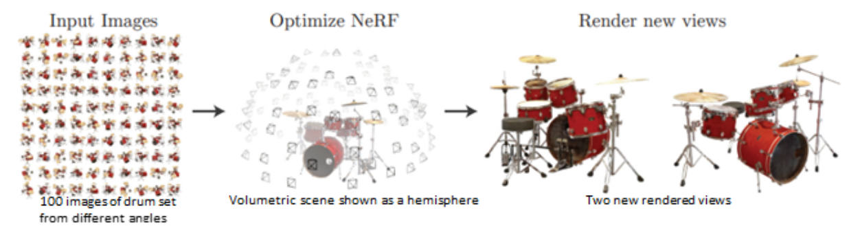
Neural Radiance Field (NeRF) 是一种从二维（2D）图像生成三维（3D）场景函数，以合成给定场景的新视图。受经典体积渲染技术的启发，NeRF 使用神经网络参数化场景函数。在本文中使用的神经网络是一个简单的多层感知器（MLP）网络。

利用从不同视角拍摄的一组场景的2D图像，可以建立一个3D函数。为此，需要使用相机参数（θ，φ）和从2D图像中采样的位置（x，y，z）来映射场景的几何结构。_视图合成_描述了可以从这个3D函数生成的新视图。体积渲染是指使用渲染技术将新视图投影到相应的2D图像上。

有多种方法可以渲染新合成的视图。最常见的两种方法是：

• 基于网格的渲染

• 体积渲染

由于损失函数的糟糕地形或陷入局部最小值，训练网格既慢又困难。而体积渲染则容易微分且易于渲染。NeRF 论文的作者优化了使用全连接网络参数化的连续体积场景函数，该网络在预测的红绿蓝（RGB）图和实际图之间的L2损失上进行了训练。与现有体积场景建模工作的成功相比，他们的方法的成功归因于：

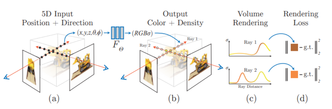
• 5D 辐射场: 模型的输入由五维（5D）坐标（三个空间单位 [x,y,z] 和两个相机方向 [θ, φ]）组成。与以前仅限于简单形状，导致过度平滑渲染的工作不同，5D辐射场使得复杂场景的映射和逼真的视图合成成为可能。给定5D输入（x, y, z, θ, φ），该模型为合成视图中的每个像素输出RGB颜色/辐射和密度。

• 位置编码（PE）: 在训练开始之前，模型对5D输入应用正弦PE。与transformers中的PE用于引入位置信息类似，NeRF使用PE来包含高频值以产生更高质量的图像。

• 分层采样和分层采样: 为了在不增加样本数量的情况下提高体积渲染的效率，从每张图像中连续采样两次点，并在两个不同的模型（粗略和精细）上进行训练。这允许筛选出与场景更相关的点，而不是周围环境。

实现

在以下章节中，我们将通过参考官方实现和Mason McGough的Colab笔记本进行端到端的NeRF训练。本实验在ROCm 5.7.0和PyTorch 2.0.1上进行。

要求

1. Install ROCm on your system在你的系统上安装ROCmInstall ROCm on your system

2. Install ROCm-compatible PyTorch安装兼容ROCm的PyTorch (卸载其他版本的PyTorch) 

数据集类

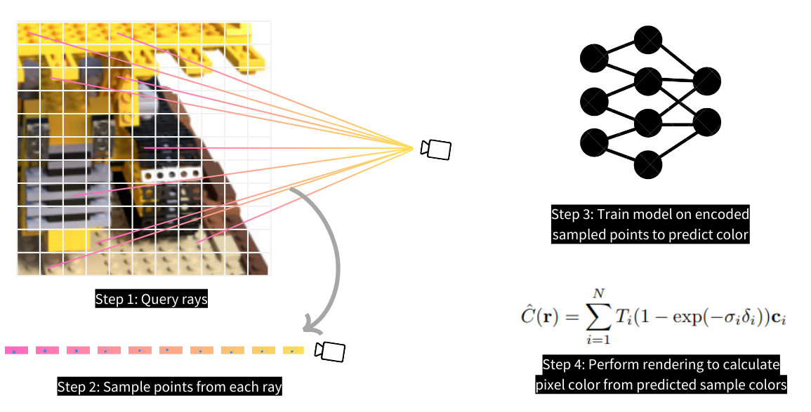
作为第一步，为您的模型准备训练数据集。与其他直接使用二维图像进行分类和检测等计算机视觉任务不同，NeRF使用多层感知器（MLP）并在从二维图像采样的位置上进行训练。准确地说，这些位置是从相机与3D场景之间的空间中采样的，如下图所示。在采样之前，您必须首先从二维图像中查询光线，然后使用分层采样技术从每条光线中采样点。

定义数据集类，该类从每张图像中查询光线。我们使用了具有106张图像及其乐高模型的相应相机姿势的[ tiny_nerf_dataset]。每个相机姿势是一个变换函数，用于将相机框架中的空间位置变换到规范设备坐标(NDC)框架中。

我们定义了一个`get_rays`函数，该函数基于图像维度（高度，宽度）和相机姿势参数化，并返回光线（起点和方向）作为输出。该函数创建了一个与输入图像相同大小的二维网格。这个网格中的每个像素表示从相机起点到该像素的一个向量（因此是负z方向）。通过焦距（即相机与投影二维图像之间的距离，通常是相机规格和一个常数值）将这些结果向量归一化到单位距离。归一化的向量通过与输入相机姿势相乘转换到NDC框架。因此，`get_rays`函数返回通过输入图像每个像素的转换光线（起点和方向）。

class NerfDataset(torch.utils.data.Dataset):def __init__(self, start_idx_dataset=0, end_idx_dataset=100):data = np.load('tiny_nerf_data.npz')self.images = torch.from_numpy(data['images'])[start_idx_dataset:end_idx_dataset]self.poses = torch.from_numpy(data['poses'])[start_idx_dataset:end_idx_dataset] # 4*4 Rotational matrix to change camera coordinates to NDC(Normalized Device Coordinates)self.focal = torch.from_numpy(data['focal']).item()def get_rays(self, pose_c2w, height=100.0, width=100.0, focal_length = 138):# 应用针孔相机模型来收集每个像素的方向i, j = torch.meshgrid(torch.arange(width),torch.arange(height),indexing='xy')directions = torch.stack([(i - width * .5) / focal_length,-(j - height * .5) / focal_length,-torch.ones_like(i) #-ve is not necessary], dim=-1)# 应用相机姿势到方向上product = directions[..., None, :] * pose_c2w[:3, :3] #(W, H, 3, 3)rays_d = torch.sum(product, dim=-1) #(W, H, 3)# 对所有方向来说，原点是相同的（光学中心）rays_o = pose_c2w[:3, -1].expand(rays_d.shape)return rays_o, rays_ddef __getitem__(self, idx):image = self.images[idx]pose = self.poses[idx]rays_o, rays_d = self.get_rays(pose, focal_length=self.focal)return rays_o, rays_d, image

分层采样

使用`stratified_sampling`函数，从每条光线上采样`n_samples=64`个点。分层采样将一条线上划分为`n_samples`个区间，并从每个区间中收集中间点。当使用扰动（`perturb`参数为非零值）时，收集的点将从每个区间的中间点略微偏移一个小的随机距离。

def stratified_sampling(rays_o, rays_d, n_samples=64, perturb=0.2):# rays_o, rays_d = self.get_rays(pose)z_vals = torch.linspace(2,6-perturb, n_samples) + torch.rand(n_samples)*perturbz_vals = z_vals.expand(list(rays_o.shape[:-1]) + [n_samples]).to('cuda') #(W,H,n_samples)# Apply scale from `rays_d` and offset from `rays_o` to samplespts = rays_o[..., None, :] + rays_d[..., None, :] * z_vals[..., :, None] #(W,H,n_samples,3)return pts.to('cuda'), z_vals.to('cuda')

位置编码

采样点和方向使用正弦编码进行编码，分别在`encode_pts`和`encode_dirs`函数中定义。随后这些编码会传递给NeRF 模型。

def encode(pts, num_freqs):freq = 2.**torch.linspace(0, num_freqs - 1, num_freqs)encoded_pts = []for i in freq:encoded_pts.append(torch.sin(pts*i))encoded_pts.append(torch.cos(pts*i))return torch.concat(encoded_pts,dim=-1)def encode_pts(pts, L=10):flattened_pts = pts.reshape(-1,3)return encode(flattened_pts, L)def encode_dirs(dirs, n_samples=64, L=4):#normalize before encodedirs = dirs / torch.norm(dirs, dim=-1, keepdim=True) #(W,H,3)dirs = dirs[..., None, :].expand(dirs.shape[:-1]+(n_samples,dirs.shape[-1])) #(W,H,num_samples,3)#print(dirs.shape)flattened_dirs = dirs.reshape((-1, 3))return encode(flattened_dirs,L)

体积渲染

NeRF模型输出每个采样点的原始颜色和密度。这些原始输出通过对每个像素的所有点进行加权求和的函数，渲染成最终图像。这个公式在论文的方程3中有描述，这里也展示了。

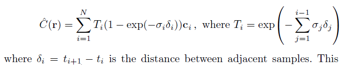
这个方程计算像素的颜色，C(r)，作为每个采样点ti在光线r上的预测颜色ci的函数。

`raw2outputs`函数返回可微分的权重和最终的颜色/辐射输出。模型在预测的RGB输出值和真实的RGB值之间的L2损失上训练。

def raw2outputs(raw: torch.Tensor,z_vals: torch.Tensor,rays_d: torch.Tensor):r"""将NeRF的原始输出转换成RGB和其他图。"""# δi = ti+1 − ti ---> (n_rays, n_samples)dists = z_vals[..., 1:] - z_vals[..., :-1]dists = torch.cat([dists, 1e10 * torch.ones_like(dists[..., :1])], dim=-1)# 归一化每个箱体的编码方向dists = dists * torch.norm(rays_d[..., None, :], dim=-1)# αi = 1 − exp(−σiδi) ---> (n_rays, n_samples)alpha = 1.0 - torch.exp(-nn.functional.relu(raw[..., 3]) * dists)# Ti(1 − exp(−σiδi)) ---> (n_rays, n_samples)# cumprod_exclusive = 指数值的乘积 = 值的和的指数**weights** = alpha * cumprod_exclusive(1. - alpha + 1e-10)# 计算加权RGB图。# 论文中的方程3rgb = torch.sigmoid(raw[..., :3])  # [n_rays, n_samples, 3]rgb_map = torch.sum(**weights**
[..., None] * rgb, dim=-2)  # [n_rays, 3]return rgb_map, **weights**

分层采样

每个输入图像会连续进行两次采样。模型在第一次前向计算（粗模型处理）中对分层样本进行处理后，在相同的输入上进行分层采样。第二次采样通过使用第一次采样中训练得到的权重来筛选出与场景更相关的3D点。模型通过创建现有权重的概率密度函数（PDF），然后从该分布中随机采样新的权重来实现这一点。

我们需要创建PDF分布的原因是为了从离散集合模拟连续值集合。然后，当随机采样新的值时，我们可以在离散点集中找到这个新值的最好/最接近的匹配。我们从分布中采样`n_samples_hierarchical=64`个权重，并通过这些新权重在离散集合中的索引从原始分层区间中提取相应的区间。以下代码片段中注释了分层采样涉及的所有步骤。

def sample_pdf(bins: torch.Tensor,weights: torch.Tensor,n_samples: int,perturb: bool = False
) -> torch.Tensor:r"""Apply inverse transform sampling to a weighted set of points."""# 规范化权重以获得PDF。# weights ---> [n_rays, n_samples]pdf = (weights + 1e-5) / torch.sum(weights + 1e-5, -1, keepdims=True) # [n_rays, n_samples]# 将PDF转换为CDF。cdf = torch.cumsum(pdf, dim=-1) # [n_rays, n_samples]cdf = torch.concat([torch.zeros_like(cdf[..., :1]), cdf], dim=-1) # [n_rays, n_samples + 1]# 随机均匀采样权重并在CDF分布中找到它们的索引。u = torch.rand(list(cdf.shape[:-1]) + [n_samples], device=cdf.device) # [n_rays, n_samples]inds = torch.searchsorted(cdf, u, right=True) # [n_rays, n_samples]# 将连续的索引堆叠为对。below = torch.clamp(inds - 1, min=0)above = torch.clamp(inds, max=cdf.shape[-1] - 1)inds_g = torch.stack([below, above], dim=-1) # [n_rays, n_samples, 2]# 从cdf中收集新权重并从现有区间中收集新区间。matched_shape = list(inds_g.shape[:-1]) + [cdf.shape[-1]] # [n_rays, n_samples, n_samples + 1]cdf_g = torch.gather(cdf.unsqueeze(-2).expand(matched_shape), dim=-1,index=inds_g) # [n_rays, n_samples, 2]bins_g = torch.gather(bins.unsqueeze(-2).expand(matched_shape), dim=-1,index=inds_g) # [n_rays, n_samples, 2]# 规范化新权重并从新区间生成分层样本。denom = (cdf_g[..., 1] - cdf_g[..., 0]) # [n_rays, n_samples]denom = torch.where(denom < 1e-5, torch.ones_like(denom), denom)t = (u - cdf_g[..., 0]) / denomsamples = bins_g[..., 0] + t * (bins_g[..., 1] - bins_g[..., 0])return samples # [n_rays, n_samples]def hierarchical_sampling(rays_o: torch.Tensor,rays_d: torch.Tensor,z_vals: torch.Tensor,weights: torch.Tensor,n_samples_hierarchical: int,perturb: bool = False
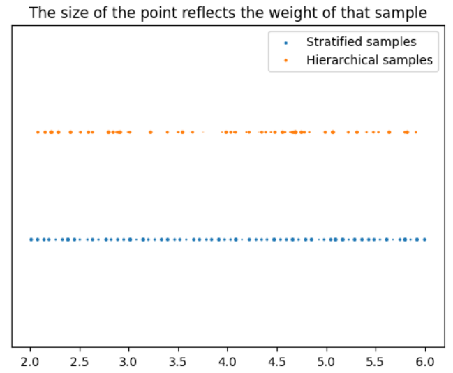
) -> Tuple[torch.Tensor, torch.Tensor, torch.Tensor]:r"""Apply hierarchical sampling to the rays."""# 使用 z_vals 作为区间和 weights 作为概率从 PDF 中抽取样本。z_vals_mid = .5 * (z_vals[..., 1:] + z_vals[..., :-1])new_z_samples = sample_pdf(z_vals_mid, weights[..., 1:-1], n_samples_hierarchical,perturb=perturb)# 使用 rays_o 和 rays_d 重新缩放点。z_vals_combined, _ = torch.sort(torch.cat([z_vals, new_z_samples], dim=-1), dim=-1)pts = rays_o[..., None, :] + rays_d[..., None, :] * z_vals_combined[..., :, None]  # [N_rays, N_samples + n_samples_hierarchical, 3]return pts.to('cuda'), z_vals_combined.to('cuda'), new_z_samples.to('cuda')

下图展示了光线上加权样本位置（包括分层样本和分层抽样样本）的可视化效果，其中光线长度在x轴上。

在第二次前向计算（精细模型处理）中，将分层样本和分层抽样样本一起传递给 NeRF model，该模型输出原始颜色。这可以使用 raw2outputs 函数进行渲染，以获得最终的RGB图。

前向传播步骤

以下代码总结了采样和训练前向步骤：

def nerf_forward(rays_o,rays_d,coarse_model,fine_model = None,n_samples=64):"""通过模型进行前向传播。"""################################################################################# 粗略模型传播################################################################################# 在每条光线上采样查询点。query_points, z_vals = stratified_sampling(rays_o, rays_d, n_samples=n_samples)encoded_points = encode_pts(query_points) # (W*H*n_samples, 60)encoded_dirs = encode_dirs(rays_d) # (W*H*n_samples, 24)raw = coarse_model(encoded_points, viewdirs=encoded_dirs)raw = raw.reshape(-1,n_samples,raw.shape[-1])# 执行可微分体积渲染以重新合成RGB图像。rgb_map, weights = raw2outputs(raw, z_vals, rays_d)outputs = {'z_vals_stratified': z_vals,'rgb_map_0': rgb_map}################################################################################# 细致模型传播################################################################################# 对细致查询点应用分层采样。query_points, z_vals_combined, z_hierarch = hierarchical_sampling(rays_o, rays_d, z_vals, weights, n_samples_hierarchical=n_samples)# 通过细致模型进行前向传播新的采样点。fine_model = fine_model if fine_model is not None else coarse_modelencoded_points = encode_pts(query_points)encoded_dirs = encode_dirs(rays_d,n_samples = n_samples*2)raw = fine_model(encoded_points, viewdirs=encoded_dirs)raw = raw.reshape(-1,n_samples*2,raw.shape[-1]) #(W*H, n_samples*2, 3+1)# 执行可微分体积渲染以重新合成RGB图像。rgb_map, weights = raw2outputs(raw, z_vals_combined, rays_d.reshape(-1, 3))# 存储输出。outputs['z_vals_hierarchical'] = z_hierarchoutputs['rgb_map'] = rgb_mapoutputs['weights'] = weightsreturn outputs

结果

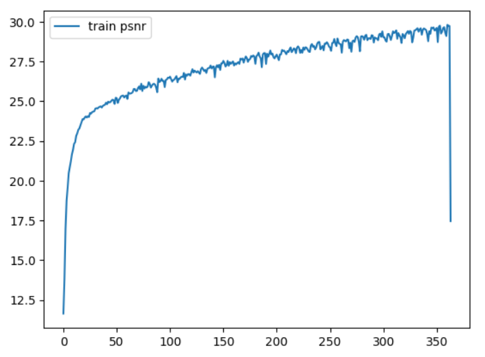
训练进行了 360 轮，并使用 Adam 优化器进行优化。整个训练大约耗时 4 小时，训练曲线如下图所示。横轴为轮次（Epochs），纵轴为峰值信噪比（PSNR），这是一个图像质量指标，值越高越好。

您可以使用 trainer.py 文件中的默认参数来复现此训练：`python trainer.py`。

您可以使用以下推理代码对测试图像生成预测。我们在代码后附上了三个测试图像的输出结果。

import torch
from dataset import stratified_sampling, encode_pts, encode_dirs, hierarchical_sampling, NerfDataset
from render import raw2outputs
from model import NeRF
from trainer import nerf_forwarddef inference(ckpt='./checkpoints/360.pt',idx=1, output_img=True):models = torch.load(ckpt)coarse_model=models['coarse']fine_model = models['fine']test_dataset = NerfDataset(100,-1)rays_o, rays_d, target_img = test_dataset[idx] # [100, 100, 3], [100, 100, 3], [100, 100, 3]rays_o, rays_d = rays_o.to('cuda'), rays_d.to('cuda')output = nerf_forward(rays_o.reshape(-1,3), rays_d.reshape(-1,3),coarse_model,fine_model,n_samples=64)if not output_img:return outputpredicted_img = output['rgb_map'].reshape(100,100,3)return predicted_img.detach().cpu().numpy()

三个测试视角的预测与相应的真实图像：

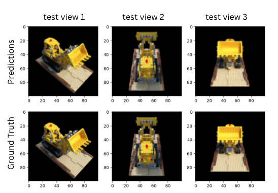
第一行显示了预测结果。第二行显示了对应的真实图像，分辨率相同，每一列对应一个特定的相机角度。