使用GPU 加速 Polars:高效解决大规模数据问题
Polars 最近新开发了一个可以支持 GPU 加速计算的执行引擎。这个引擎可以对超过 100GB 的数据进行交互式操作能。本文将详细讨论 Polars 中DF的概念、GPU 加速如何与 Polars DF协同工作,以及使用新的 CUDA 驱动执行引擎可能带来的性能提升。

Polars 核心概念
Polars 的核心功能是创建和操作DF,这些DF可以被视为具有高级功能的电子表格。以下是一个简单的示例,包含了一些人的姓名、年龄和所在城市信息:
""" 在 Polars 中创建一个简单的DF """ importpolarsaspl df=pl.DataFrame({ "name": ["Alice", "Bob", "Charlie", "Jill", "William"], "age": [25, 30, 35, 22, 40], "city": ["New York", "Los Angeles", "Chicago", "New York", "Chicago"] }) print(df)
输出结果:
shape: (5, 3)┌─────────┬─────┬─────────────┐│ name ┆ age ┆ city ││ --- ┆ --- ┆ --- ││ str ┆ i64 ┆ str │╞═════════╪═════╪═════════════╡│ Alice ┆ 25 ┆ New York ││ Bob ┆ 30 ┆ Los Angeles ││ Charlie ┆ 35 ┆ Chicago ││ Jill ┆ 22 ┆ New York ││ William ┆ 40 ┆ Chicago │└─────────┴─────┴─────────────┘
使用这个DF,我们可以执行多种操作,例如按年龄筛选:
""" 筛选上述DF,仅显示年龄超过 28 的行 """ df_filtered=df.filter(pl.col("age") >28) print(df_filtered)
输出结果:
shape: (3, 3) ┌─────────┬─────┬─────────────┐ │ name ┆ age ┆ city │ │ --- ┆ --- ┆ --- │ │ str ┆ i64 ┆ str │ ╞═════════╪═════╪═════════════╡ │ Bob ┆ 30 ┆ Los Angeles │ │ Charlie ┆ 35 ┆ Chicago │ │ William ┆ 40 ┆ Chicago │ └─────────┴─────┴─────────────┘
我们还可以进行数学运算:
""" 创建一个名为 "age_doubled" 的新列,其值为 age 列的两倍 """ df=df.with_columns([ (pl.col("age") *2).alias("age_doubled") ]) print(df)
输出结果:
shape: (5, 4) ┌─────────┬─────┬─────────────┬─────────────┐ │ name ┆ age ┆ city ┆ age_doubled │ │ --- ┆ --- ┆ --- ┆ --- │ │ str ┆ i64 ┆ str ┆ i64 │ ╞═════════╪═════╪═════════════╪═════════════╡ │ Alice ┆ 25 ┆ New York ┆ 50 │ │ Bob ┆ 30 ┆ Los Angeles ┆ 60 │ │ Charlie ┆ 35 ┆ Chicago ┆ 70 │ │ Jill ┆ 22 ┆ New York ┆ 44 │ │ William ┆ 40 ┆ Chicago ┆ 80 │ └─────────┴─────┴─────────────┴─────────────┘
也可以执行聚合函数,如计算每个城市的平均年龄:
""" 按城市计算平均年龄 """ df_aggregated=df.group_by("city").agg(pl.col("age").mean()) print(df_aggregated)
输出结果:
shape: (3, 2) ┌─────────────┬──────┐ │ city ┆ age │ │ --- ┆ --- │ │ str ┆ f64 │ ╞═════════════╪══════╡ │ Chicago ┆ 37.5 │ │ New York ┆ 23.5 │ │ Los Angeles ┆ 30.0 │ └─────────────┴──────┘
对于熟悉 Pandas 的读者来说,Polars 可能看起来很相似。但是Polars 具有一些独特的特性,使其在某些情况下更为高效。在深入探讨 GPU 加速的 Polars 之前,我们先来了解一下 Polars 的一个关键特性:LazyFrames。
Polars LazyFrames
Polars 提供了两种基本的执行模式:“eager”(急切)和"lazy"(惰性)。Eager DF在调用时立即执行计算,完全按照指定的方式进行。例如,对一个列的每个值加 2,然后再加 3,这些操作会按照你期望的顺序立即执行。
让我们通过一个示例来对比 eager 和 lazy 执行模式:
import polars as pl  # 创建一个包含数字列表的 DataFrame
df = pl.DataFrame({  "numbers": [1, 2, 3, 4, 5]
})  # 对每个数字加 2,并覆盖原始的 'numbers' 列
df = df.with_columns(  pl.col("numbers") + 2
)  # 对更新后的 'numbers' 列再加 3
df = df.with_columns(  pl.col("numbers") + 3
)  print(df)
输出结果:
shape: (5, 1)
┌─────────┐
│ numbers │
│ ---     │
│ i64     │
╞═════════╡
│ 6       │
│ 7       │
│ 8       │
│ 9       │
│ 10      │
└─────────┘
现在,让我们使用
.lazy()
函数来初始化一个惰性操作:
import polars as pl  # 创建一个惰性 DataFrame,包含数字列表
df = pl.DataFrame({  "numbers": [1, 2, 3, 4, 5]
}).lazy() # <-------------------------- 惰性初始化  # 对每个数字加 2,并覆盖原始的 'numbers' 列
df = df.with_columns(  pl.col("numbers") + 2
)  # 对更新后的 'numbers' 列再加 3
df = df.with_columns(  pl.col("numbers") + 3
)  print(df)
输出结果:
naive plan: (run LazyFrame.explain(optimized=True) to see the optimized plan) WITH_COLUMNS: [[(col("numbers")) + (3)]] WITH_COLUMNS: [[(col("numbers")) + (2)]] DF ["numbers"]; PROJECT */1 COLUMNS; SELECTION: "None"
在这个惰性执行模式下,我们得到的不是一个DF,而是一个类似 SQL 的表达式,它概述了需要执行哪些操作才能得到我们想要的DF。要实际执行这些计算并获得结果,我们需要调用
.collect()
方法:
print(df.collect())
输出结果:
shape: (5, 1)
┌─────────┐
│ numbers │
│ ---     │
│ i64     │
╞═════════╡
│ 6       │
│ 7       │
│ 8       │
│ 9       │
│ 10      │
└─────────┘
惰性执行的优势不在于计算发生的时间,而在于实际执行的计算内容。在执行惰性DF之前,Polars 会分析累积的操作,并寻找可能提高执行效率的优化路径。这个过程被称为"查询优化"。
让我们通过一个更复杂的例子来说明这一点:
# 创建一个包含多个列的 DataFrame
df = pl.DataFrame({  "col_0": [1, 2, 3, 4, 5],  "col_1": [8, 7, 6, 5, 4],  "col_2": [-1, -2, -3, -4, -5]
}).lazy()  # 执行一些随机操作
df = df.filter(pl.col("col_0") > 0)
df = df.with_columns((pl.col("col_1") * 2).alias("col_1_double"))
df = df.group_by("col_2").agg(pl.sum("col_1_double"))  print(df)
输出结果:
naive plan: (run LazyFrame.explain(optimized=True) to see the optimized plan) AGGREGATE [col("col_1_double").sum()] BY [col("col_2")] FROM WITH_COLUMNS: [[(col("col_1")) * (2)].alias("col_1_double")] FILTER [(col("col_0")) > (0)] FROM DF ["col_0", "col_1", "col_2"]; PROJECT */3 COLUMNS; SELECTION: "None"
现在,让我们看看优化后的执行计划:
print(df.explain(optimized=True))
输出结果:
AGGREGATE [col("col_1_double").sum()] BY [col("col_2")] FROM WITH_COLUMNS: [[(col("col_1")) * (2)].alias("col_1_double")] DF ["col_0", "col_1", "col_2"]; PROJECT */3 COLUMNS; SELECTION: "[(col(\"col_0\")) > (0)]"
这个优化后的表达式就是在调用
.collect()
方法时实际执行的内容。
为了量化惰性执行带来的性能提升,我们可以进行一个简单的性能测试,比较 eager 和 lazy 执行模式的速度差异:
import polars as pl
import numpy as np
import time  # 设定常量
num_rows = 20_000_000  # 2千万行
num_cols = 10          # 10列
n = 10  # 测试重复次数  # 生成随机数据
np.random.seed(0)  # 设置随机种子以确保可重复性
data = {f"col_{i}": np.random.randn(num_rows) for i in range(num_cols)}  # 定义一个适用于 lazy 和 eager DataFrame 的函数
def apply_transformations(df):  df = df.filter(pl.col("col_0") > 0)  # 筛选 col_0 大于 0 的行  df = df.with_columns((pl.col("col_1") * 2).alias("col_1_double"))  # 将 col_1 乘以 2  df = df.group_by("col_2").agg(pl.sum("col_1_double"))  # 按 col_2 分组并聚合  return df  # 存储 eager 和 lazy 执行的总持续时间的变量
total_eager_duration = 0
total_lazy_duration = 0  # 执行 n 次测试
for i in range(n):  print(f"运行 {i+1}/{n}")  # 为每次运行创建新的 DataFrame(polars 操作可能是原地的,所以确保 DF 是干净的)  df1 = pl.DataFrame(data)  df2 = pl.DataFrame(data).lazy()  # 测量 eager 执行时间  start_time_eager = time.time()  eager_result = apply_transformations(df1)  # Eager 执行  eager_duration = time.time() - start_time_eager  total_eager_duration += eager_duration  print(f"Eager 执行时间: {eager_duration:.2f} 秒")  # 测量 lazy 执行时间  start_time_lazy = time.time()  lazy_result = apply_transformations(df2).collect()  # Lazy 执行  lazy_duration = time.time() - start_time_lazy  total_lazy_duration += lazy_duration  print(f"Lazy 执行时间: {lazy_duration:.2f} 秒")  # 计算平均执行时间
average_eager_duration = total_eager_duration / n
average_lazy_duration = total_lazy_duration / n  # 计算 lazy 执行比 eager 执行快多少
faster = (average_eager_duration-average_lazy_duration)/average_eager_duration*100  print(f"\n{n} 次运行的平均 Eager 执行时间: {average_eager_duration:.2f} 秒")
print(f"{n} 次运行的平均 Lazy 执行时间: {average_lazy_duration:.2f} 秒")
print(f"Lazy 执行节省了 {faster:.2f}% 的时间")
输出结果:
运行 1/10
Eager 执行时间: 3.07 秒
Lazy 执行时间: 2.70 秒
运行 2/10
Eager 执行时间: 4.17 秒
Lazy 执行时间: 2.69 秒
运行 3/10
Eager 执行时间: 2.97 秒
Lazy 执行时间: 2.76 秒
运行 4/10
Eager 执行时间: 4.21 秒
Lazy 执行时间: 2.74 秒
运行 5/10
Eager 执行时间: 2.97 秒
Lazy 执行时间: 2.77 秒
运行 6/10
Eager 执行时间: 4.12 秒
Lazy 执行时间: 2.80 秒
运行 7/10
Eager 执行时间: 3.00 秒
Lazy 执行时间: 2.72 秒
运行 8/10
Eager 执行时间: 4.53 秒
Lazy 执行时间: 2.76 秒
运行 9/10
Eager 执行时间: 3.14 秒
Lazy 执行时间: 3.08 秒
运行 10/10
Eager 执行时间: 4.26 秒
Lazy 执行时间: 2.77 秒  10 次运行的平均 Eager 执行时间: 3.64 秒
10 次运行的平均 Lazy 执行时间: 2.78 秒
Lazy 执行节省了 23.75% 的时间
这个 23.75% 的性能提升是相当可观的,这种提升是通过惰性执行实现的,而这在 Pandas 中是不存在的。在底层当使用 Polars 惰性DF时,实际上是在定义一个高级计算图,Polars 会对其进行各种优化处理。在优化查询之后再执行,这意味着你会得到与 eager DF相同的结果,但通常速度更快。

上图是 Polars 中调用查询后触发的操作的高级概述。eager 执行本身就有许多优化改进,如原生多核支持,这在惰性执行中也存在并得到了进一步改进。
尽管 Lazy 执行模式带来了显著的性能提升,但对于一些用户来说,这种提升可能还不足以促使他们改变长期使用的工具。接下来我们将介绍的 GPU 加速功能可能会彻底改变这种看法。
GPU 加速 Polars
GPU 加速功能是 Polars 最新引入的特性。在撰写本文时,这项功能刚刚发布。要在环境中启用 GPU 加速,可以使用以下命令安装支持 GPU 的 Polars:
pip install polars[gpu] --extra-index-url=https://pypi.nvidia.com
如果上述命令不起作用,建议查看 Polars 的 PyPI 页面以获取最新的安装说明。
启用 GPU 加速后,只需在调用
collect()
方法时指定 GPU 作为执行引擎即可使用 GPU 加速功能。具体实现如下:
gpu_engine = pl.GPUEngine(device=0,  # 默认设置raise_on_fail=True,  # 如果无法在 GPU 上运行,则抛出异常
)results = df.collect(engine=gpu_engine)
但是GPU 执行引擎并不支持所有的 Polars 功能。如果遇到不支持的操作,默认情况下会回退到 CPU 执行。通过设置
raise_on_fail=True
,我们可以在不支持 GPU 执行时得到明确的错误提示。
为了量化 GPU 加速带来的性能提升,我们可以进行一个更全面的性能测试,比较 eager 执行、CPU 上的 lazy 执行和 GPU 上的 lazy 执行:
import polars as pl
import numpy as np
import time# 创建大型随机 DataFrame
num_rows = 20_000_000  # 2千万行
num_cols = 10          # 10列
n = 10  # 测试重复次数# 生成随机数据
np.random.seed(0)  # 设置随机种子以确保可重复性
data = {f"col_{i}": np.random.randn(num_rows) for i in range(num_cols)}# 定义适用于 lazy 和 eager DataFrame 的函数
def apply_transformations(df):df = df.filter(pl.col("col_0") > 0)  # 筛选 col_0 大于 0 的行df = df.with_columns((pl.col("col_1") * 2).alias("col_1_double"))  # 将 col_1 乘以 2df = df.group_by("col_2").agg(pl.sum("col_1_double"))  # 按 col_2 分组并聚合return df# 存储执行时间的变量
total_eager_duration = 0
total_lazy_duration = 0
total_lazy_GPU_duration = 0# 执行 n 次测试
for i in range(n):print(f"运行 {i+1}/{n}")# 为每次运行创建新的 DataFramedf1 = pl.DataFrame(data)df2 = pl.DataFrame(data).lazy()df3 = pl.DataFrame(data).lazy()# 测量 eager 执行时间start_time_eager = time.time()eager_result = apply_transformations(df1)  # Eager 执行eager_duration = time.time() - start_time_eagertotal_eager_duration += eager_durationprint(f"Eager 执行时间: {eager_duration:.2f} 秒")# 测量 CPU lazy 执行时间start_time_lazy = time.time()lazy_result = apply_transformations(df2).collect()  # CPU Lazy 执行lazy_duration = time.time() - start_time_lazytotal_lazy_duration += lazy_durationprint(f"CPU Lazy 执行时间: {lazy_duration:.2f} 秒")# 定义 GPU 引擎gpu_engine = pl.GPUEngine(device=0,  # 默认设置raise_on_fail=True,  # 如果无法在 GPU 上运行,则抛出异常)# 测量 GPU lazy 执行时间start_time_lazy_GPU = time.time()lazy_result = apply_transformations(df3).collect(engine=gpu_engine)  # GPU Lazy 执行lazy_GPU_duration = time.time() - start_time_lazy_GPUtotal_lazy_GPU_duration += lazy_GPU_durationprint(f"GPU Lazy 执行时间: {lazy_GPU_duration:.2f} 秒")# 计算平均执行时间
average_eager_duration = total_eager_duration / n
average_lazy_duration = total_lazy_duration / n
average_lazy_GPU_duration = total_lazy_GPU_duration / n# 计算性能提升
faster_1 = (average_eager_duration-average_lazy_duration)/average_eager_duration*100
faster_2 = (average_lazy_duration-average_lazy_GPU_duration)/average_lazy_duration*100
faster_3 = (average_eager_duration-average_lazy_GPU_duration)/average_eager_duration*100print(f"\n{n} 次运行的平均 Eager 执行时间: {average_eager_duration:.2f} 秒")
print(f"{n} 次运行的平均 CPU Lazy 执行时间: {average_lazy_duration:.2f} 秒")
print(f"{n} 次运行的平均 GPU Lazy 执行时间: {average_lazy_GPU_duration:.2f} 秒")
print(f"CPU Lazy 比 Eager 快 {faster_1:.2f}%")
print(f"GPU 比 CPU Lazy 快 {faster_2:.2f}%,比 Eager 快 {faster_3:.2f}%")
输出结果:
运行 1/10
Eager 执行时间: 0.74 秒
CPU Lazy 执行时间: 0.66 秒
GPU Lazy 执行时间: 0.17 秒
运行 2/10
Eager 执行时间: 0.72 秒
CPU Lazy 执行时间: 0.65 秒
GPU Lazy 执行时间: 0.17 秒
运行 3/10
Eager 执行时间: 0.82 秒
CPU Lazy 执行时间: 0.76 秒
GPU Lazy 执行时间: 0.17 秒
运行 4/10
Eager 执行时间: 0.81 秒
CPU Lazy 执行时间: 0.69 秒
GPU Lazy 执行时间: 0.18 秒
运行 5/10
Eager 执行时间: 0.79 秒
CPU Lazy 执行时间: 0.66 秒
GPU Lazy 执行时间: 0.18 秒
运行 6/10
Eager 执行时间: 0.75 秒
CPU Lazy 执行时间: 0.63 秒
GPU Lazy 执行时间: 0.18 秒
运行 7/10
Eager 执行时间: 0.77 秒
CPU Lazy 执行时间: 0.72 秒
GPU Lazy 执行时间: 0.18 秒
运行 8/10
Eager 执行时间: 0.77 秒
CPU Lazy 执行时间: 0.72 秒
GPU Lazy 执行时间: 0.17 秒
运行 9/10
Eager 执行时间: 0.77 秒
CPU Lazy 执行时间: 0.72 秒
GPU Lazy 执行时间: 0.17 秒
运行 10/10
Eager 执行时间: 0.77 秒
CPU Lazy 执行时间: 0.70 秒
GPU Lazy 执行时间: 0.17 秒10 次运行的平均 Eager 执行时间: 0.77 秒
10 次运行的平均 CPU Lazy 执行时间: 0.69 秒
10 次运行的平均 GPU Lazy 执行时间: 0.17 秒
CPU Lazy 比 Eager 快 10.30%
GPU 比 CPU Lazy 快 74.78%,比 Eager 快 77.38%
这些结果显示,GPU 加速带来了显著的性能提升。GPU 执行比 CPU 上的 lazy 执行快了 74.78%,比 eager 执行快了 77.38%。这还不是一个特别大的数据集。对于更大的数据集,我们可能会看到更显著的性能提升。
GPU 加速的工作原理
Polars 的 GPU 加速功能是通过添加一个新的 GPU 执行引擎实现的。这个新引擎与现有的执行引擎并存,Polars 可以根据可用的硬件和正在执行的查询类型动态选择最适合的引擎。
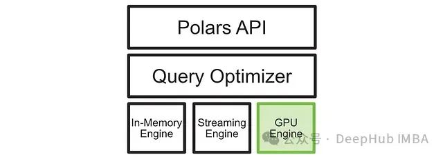
如上图所示,在输入查询后,查询优化器会优化查询,并将操作发送到最合适的执行引擎。新增的 GPU 执行引擎为高度可并行化的操作提供了显著的性能提升。
一些查询在 GPU 上表现极佳,而其他查询可能仍然在 CPU 上使用内存引擎完成。这种灵活的设计使得 CUDA 加速的 Polars 在大多数情况下都能提供更快的执行速度,特别是在处理大型数据集时。
抽象的内存管理
Nvidia 和 Polars 团队在设计新的查询优化器时,特别关注了 CPU 和 GPU 之间的内存管理问题。对于不熟悉 GPU 编程的读者来说,需要了解 CPU 和 GPU 使用不同的内存系统:CPU 使用主机内存(RAM),而 GPU 使用设备内存(VRAM)。
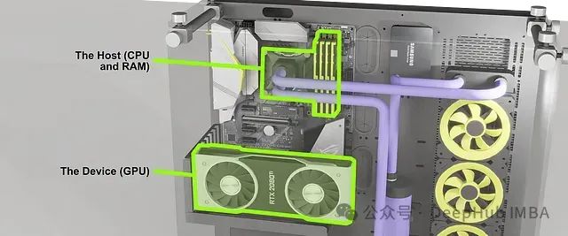
如上图所示,CPU 和 GPU 可以看作是两个独立的计算单元,各自拥有自己的资源,并通过特定的接口进行通信。CPU 进行通用计算并使用 RAM 存储数据,而 GPU 专门进行并行计算,使用显卡上的 VRAM 存储数据。在复杂的数据处理任务中,这两个系统需要协同工作。
Polars 的查询优化器能够智能地处理 CPU 和 GPU 之间的数据传输。例如当一个在 GPU 上创建和执行的DF需要与仍在 CPU 上的另一个DF交互时,查询优化器可以自动处理必要的数据传输。
这种抽象的内存管理为用户提供了极大的便利,使得在 GPU 上进行数据处理变得简单直接。然而对于一些特定的工作流程,如同时进行大规模数据操作和模型训练的场景,这种自动化的内存管理可能会带来一些挑战。在这些情况下可能需要更精细的内存控制。
Nvidia 和 Polars 团队正在研究显式内存控制功能,这可能会在未来的版本中推出。对于纯数据处理工作负载,当前的自动内存管理机制已经能够为大多数数据科学家和工程师节省大量时间。
总结
GPU 加速 Polars 的引入为数据处理领域带来了令人兴奋的新可能性。这项技术不仅提供了显著的性能提升,还保持了 Polars 易用和灵活的特性。
尽管对于一些简单的数据处理任务,传统工具如 Pandas 可能仍然足够,但在面对大型数据集和复杂查询时,GPU 加速的 Polars 显示出了巨大的优势。其提供的性能提升可能会影响许多数据科学家和工程师的工作流程,使得previously耗时的操作变得更加高效。
随着这项技术的进一步发展和完善,我们可以期待看到更多创新的数据处理应用场景。对于那些经常处理大规模数据的专业人士来说,密切关注 Polars 和 GPU 加速数据处理技术的发展将是十分有益的。
https://avoid.overfit.cn/post/b9974462d508445d821aef4f471793fe