pytorch学习使用
1. 基础使用
1.1 基础信息
# 输出 torch 版本
print(torch.__version__)# 判断 cuda 是否可用
print(torch.cuda.is_available())
"""
2.7.0
False
"""
1.2 创建tensor
# 创建一个5*3的矩阵,初始值为0.
print("-------- empty --------")
print(torch.empty(5, 3))  # 等价与 torch.empty((5, 3))# 创建一个随机初始化的 5*3 矩阵,初始值在[0, 1)之间,符合均匀分布
print("-------- rand --------")
rand_x = torch.rand(5, 3)  # 等价于 rand_x = torch.rand((5, 3))
print(rand_x)
print(rand_x[:, 0]) # 访问第0列,输出为一维数组
print(rand_x[0, :]) # 访问第0行,输出为一维数组
print(rand_x[:, 0:2]) # 访问前两列,输出为二维数组
print(rand_x[:, [0, 2]]) # 访问第0列,第2列,输出为二维数组
print(rand_x[::2]) # 第0,2,4行,输出为二维数组# 创建一个随机初始化的 2*10 矩阵,符合标准正态分布
print("-------- normal --------")
normal_x = torch.normal(0, 1, size=(2, 10))
print(normal_x)# 创建一个随机初始化的一维矩阵,初始值在[0, 1000)之间
print("-------- randint --------")
randint_x = torch.randint(low=0, high=1000, size=(8,))
print(randint_x)# 创建一个数值皆是 0,类型为 long 的矩阵
print("-------- zeros --------")
zero_x = torch.zeros(5, 3, dtype=torch.long)  # 等价于 zero_x = torch.zeros((5, 3), dtype=torch.long)
print(zero_x)# 创建一个数值皆是 1. ,类型为 float 的矩阵
print("-------- ones --------")
one_x = torch.ones(5, 3, dtype=torch.float)  # 等价于 zero_x = torch.ones((5, 3), dtype=torch.float)
print(one_x)# 创建一个对角线数值皆是 1. ,类型为 float 的矩阵
print("-------- eye --------")
eye_x = torch.eye(5, 3, dtype=torch.float)
print(eye_x)
# 提取对角线元素
s = eye_x.diag()
print(s)
# 将向量嵌入对角线生成矩阵
t = s.diag_embed() # 等价于:t = torch.diag_embed(s)
print(t)# 创建一维tensor 数值是 [5.5, 3],值中有一个浮点数,因此所有数值均为浮点类型
print("-------- 一维tensor --------")
tensor1 = torch.tensor([5.5, 3])
print(tensor1)# 创建二维tensor,值中无浮点数,因此所有数值均为整数类型
print("-------- 二维tensor --------")
tensor0 = torch.tensor([[1, 2], [3, 4], [5, 6]])
print(tensor0)# 基于现有张量,创建一个新张量,其形状由参数 size 定义,所有元素值为1,默认继承原张量的数据类型(dtype)和设备(如CPU/GPU)
print("-------- new_ones --------")
tensor2 = tensor1.new_ones((2, 3))
print(tensor2)# 修改数值类型
print("-------- randn_like --------")
tensor3 = torch.randn_like(tensor2, dtype=torch.float)
print(tensor3)# 输出 tensor 的 size
print("-------- tensor size --------")
print(tensor3.size())
print(tensor3.shape)# 将单元素张量转化为python标量
print("-------- tensor item --------")
tensor4 = torch.Tensor([3.14])
print(tensor4.item())
"""
-------- empty --------
tensor([[0., 0., 0.],[0., 0., 0.],[0., 0., 0.],[0., 0., 0.],[0., 0., 0.]])
-------- rand --------
tensor([[0.6596, 0.3999, 0.4556],[0.2757, 0.6820, 0.7506],[0.0683, 0.1522, 0.9666],[0.7557, 0.1943, 0.2406],[0.5978, 0.7308, 0.1105]])
tensor([0.6596, 0.2757, 0.0683, 0.7557, 0.5978])
tensor([0.6596, 0.3999, 0.4556])
tensor([[0.6596, 0.3999],[0.2757, 0.6820],[0.0683, 0.1522],[0.7557, 0.1943],[0.5978, 0.7308]])
tensor([[0.6596, 0.4556],[0.2757, 0.7506],[0.0683, 0.9666],[0.7557, 0.2406],[0.5978, 0.1105]])
tensor([[0.6596, 0.3999, 0.4556],[0.0683, 0.1522, 0.9666],[0.5978, 0.7308, 0.1105]])
-------- normal --------
tensor([[ 0.3300, -0.5461,  1.3952, -1.4907, -0.4039,  0.2111,  0.4386,  0.6213,-0.9563, -0.4214],[-0.2401, -1.3838, -1.1084,  1.8060, -0.1078, -0.1417, -1.5372, -0.3526,0.2074, -1.0423]])
-------- randint --------
tensor([474, 834, 908, 552, 926, 543, 338, 452])
-------- zeros --------
tensor([[0, 0, 0],[0, 0, 0],[0, 0, 0],[0, 0, 0],[0, 0, 0]])
-------- ones --------
tensor([[1., 1., 1.],[1., 1., 1.],[1., 1., 1.],[1., 1., 1.],[1., 1., 1.]])
-------- eye --------
tensor([[1., 0., 0.],[0., 1., 0.],[0., 0., 1.],[0., 0., 0.],[0., 0., 0.]])
tensor([1., 1., 1.])
tensor([[1., 0., 0.],[0., 1., 0.],[0., 0., 1.]])
-------- 一维tensor --------
tensor([5.5000, 3.0000])
-------- 二维tensor --------
tensor([[1, 2],[3, 4],[5, 6]])
-------- new_ones --------
tensor([[1., 1., 1.],[1., 1., 1.]])
-------- randn_like --------
tensor([[ 0.4086,  0.6232, -0.6118],[ 0.3720,  0.0189,  1.0114]])
-------- tensor size --------
torch.Size([2, 3])
torch.Size([2, 3])
-------- tensor item --------
3.140000104904175
"""
1.3 tensor之间的运算
a = torch.tensor([[1.0, 2, 3], [4, 5, 6]])
b = torch.tensor([[1, 2, 3], [4, 5, 6]])
# 加法
print("-------- tensor之间相加 --------")
c = a + b
print(c)
c = torch.add(a, b)
print(c)
c = a.add(b)
print(c)
# a.add_(b) # 会修改a的值,最后带下划线的都会修改调用者的值
# print(a)# 减法
print("-------- tensor之间相减 --------")
c = a - b
print(c)
c = torch.sub(a, b)
print(c)
c = a.sub(b)
print(c)
# a.sub_(b) # 会修改a的值,最后带下划线的都会修改调用者的值
# print(a)# 乘法,哈达玛积(对应元素相乘)
print("-------- tensor之间相乘 --------")
c = a * b
print(c)
c = torch.mul(a, b)
print(c)
c = a.mul(b)
print(c)
# a.mul_(b) # 会修改a的值,最后带下划线的都会修改调用者的值
# print(a)# 除法
print("-------- tensor之间相除 --------")
c = a / b
print(c)
c = torch.div(a, b)
print(c)
c = a.div(b)
print(c)
# a.div_(b) # 会修改a的值,最后带下划线的都会修改调用者的值,a必须是浮点数类型
# print(a)# 矩阵乘法
print("-------- tensor之间矩阵乘法 --------")
a = torch.tensor([[1, 1, 1], [1, 1, 1]])
b = torch.tensor([[1, 1], [1, 1], [1, 1]])
c = torch.mm(a, b)
print(c)
c = torch.matmul(a, b)
print(c)
c = a @ b
print(c)
c = a.matmul(b)
print(c)# 幂运算
print("-------- tensor幂运算 --------")
a = torch.tensor([[1, 2, 3], [4, 5, 6]])
c = torch.pow(a, 3)
print(c)
c = a.pow(3)
print(c)
c = a**3
print(c)
# a.pow_(3) # 会修改a的值,最后带下划线的都会修改调用者的值
# print(a)# 开方运算
print("-------- tensor幂运算 --------")
a = torch.tensor([[1.0, 2, 3], [4, 5, 6]])
c = a.sqrt()
print(c)
# a.sqrt_() # 会修改a的值,最后带下划线的都会修改调用者的值,a必须是浮点数类型
# print(a)# 对数
print("-------- tensor对数运算 --------")
a = torch.tensor([[1.0, 2, 3], [4, 5, 6]])
c = torch.log2(a)
print(c)
c = torch.log10(a)
print(c)
c = torch.log(a) # 以e为底
print(c)
# torch.log_(a) # 会修改a的值,最后带下划线的都会修改调用者的值,a必须是浮点数类型
# print(a)
"""
-------- tensor之间相加 --------
tensor([[ 2.,  4.,  6.],[ 8., 10., 12.]])
tensor([[ 2.,  4.,  6.],[ 8., 10., 12.]])
tensor([[ 2.,  4.,  6.],[ 8., 10., 12.]])
-------- tensor之间相减 --------
tensor([[0., 0., 0.],[0., 0., 0.]])
tensor([[0., 0., 0.],[0., 0., 0.]])
tensor([[0., 0., 0.],[0., 0., 0.]])
-------- tensor之间相乘 --------
tensor([[ 1.,  4.,  9.],[16., 25., 36.]])
tensor([[ 1.,  4.,  9.],[16., 25., 36.]])
tensor([[ 1.,  4.,  9.],[16., 25., 36.]])
-------- tensor之间相除 --------
tensor([[1., 1., 1.],[1., 1., 1.]])
tensor([[1., 1., 1.],[1., 1., 1.]])
tensor([[1., 1., 1.],[1., 1., 1.]])
-------- tensor之间矩阵乘法 --------
tensor([[3, 3],[3, 3]])
tensor([[3, 3],[3, 3]])
tensor([[3, 3],[3, 3]])
tensor([[3, 3],[3, 3]])
-------- tensor幂运算 --------
tensor([[  1,   8,  27],[ 64, 125, 216]])
tensor([[  1,   8,  27],[ 64, 125, 216]])
tensor([[  1,   8,  27],[ 64, 125, 216]])
-------- tensor幂运算 --------
tensor([[1.0000, 1.4142, 1.7321],[2.0000, 2.2361, 2.4495]])
-------- tensor对数运算 --------
tensor([[0.0000, 1.0000, 1.5850],[2.0000, 2.3219, 2.5850]])
tensor([[0.0000, 0.3010, 0.4771],[0.6021, 0.6990, 0.7782]])
tensor([[0.0000, 0.6931, 1.0986],[1.3863, 1.6094, 1.7918]])
"""
1.4 tensor和数字之间的运算
a = torch.tensor([[1.0, 2, 3], [4, 5, 6]])
b = 2# 加减乘除,tensor中的每个数字都与b进行运算
print(a + b)
print(a - b)
print(a * b)
print(a / b)
"""
tensor([[3., 4., 5.],[6., 7., 8.]])
tensor([[-1.,  0.,  1.],[ 2.,  3.,  4.]])
tensor([[ 2.,  4.,  6.],[ 8., 10., 12.]])
tensor([[0.5000, 1.0000, 1.5000],[2.0000, 2.5000, 3.0000]])
"""
1.5 tensor尺寸修改
print("-------- 二维张量 --------")
a = torch.tensor([[1.0, 2, 3, 4], [5, 6, 7, 8], [9, 10, 11, 12]])
c = a.reshape(-1, 2) # 转化成两列的二维矩阵
print(c)
c = a.view(-1, 3) # 转化成三列的二维矩阵
print(c)
c = a.reshape(-1) # 按照行转化为一维数组
print(c)
c = a.view(-1) # 按照行转化为一维数组
print(c)
print("-------- 三维维张量 --------")
a = torch.tensor([[[1.0, 2, 3],[4, 5, 6],[7, 8, 9]],[[10, 11, 12],[13, 14, 15],[16, 17, 18]],[[20, 21, 22],[23, 24, 25],[26, 27, 28]]
])
c = a.view(-1, 3*3)
print(c)
"""
-------- 二维张量 --------
tensor([[ 1.,  2.],[ 3.,  4.],[ 5.,  6.],[ 7.,  8.],[ 9., 10.],[11., 12.]])
tensor([[ 1.,  2.,  3.],[ 4.,  5.,  6.],[ 7.,  8.,  9.],[10., 11., 12.]])
tensor([ 1.,  2.,  3.,  4.,  5.,  6.,  7.,  8.,  9., 10., 11., 12.])
tensor([ 1.,  2.,  3.,  4.,  5.,  6.,  7.,  8.,  9., 10., 11., 12.])
-------- 三维维张量 --------
tensor([[ 1.,  2.,  3.,  4.,  5.,  6.,  7.,  8.,  9.],[10., 11., 12., 13., 14., 15., 16., 17., 18.],[20., 21., 22., 23., 24., 25., 26., 27., 28.]])
"""
1.6 tensor转置
print("-------- 一维张量 --------")
a = torch.tensor([1, 2, 3])  # shape: (3,)
c = a.transpose(0, 0)  # 无变化,仍为 [1, 2, 3]
print(c)
b = a.unsqueeze(0)  # shape: (1, 3),先通过 unsqueeze() 升维至二维,再转置
c = b.transpose(0, 1)  # shape: (3, 1)
print(c)print("-------- 二维张量 --------")
a = torch.tensor([[1, 2], [3, 4], [5, 6]])  # shape: (3, 2)
c = a.transpose(0, 1)  # 或 a.t()
print(a)
print(c)  # tensor([[1, 3, 5], [2, 4, 6]]), shape: (2, 3)
c = a.t()
print(c)print("-------- 三维张量 --------")
a = torch.arange(24).reshape(2, 3, 4)  # shape: (2, 3, 4)
c = a.transpose(0, 2)  # 交换第0和第2维
print(a)
print(c) # torch.Size([4, 3, 2])
"""
-------- 一维张量 --------
tensor([1, 2, 3])
tensor([[1],[2],[3]])
-------- 二维张量 --------
tensor([[1, 2],[3, 4],[5, 6]])
tensor([[1, 3, 5],[2, 4, 6]])
tensor([[1, 3, 5],[2, 4, 6]])
-------- 三维张量 --------
tensor([[[ 0,  1,  2,  3],[ 4,  5,  6,  7],[ 8,  9, 10, 11]],[[12, 13, 14, 15],[16, 17, 18, 19],[20, 21, 22, 23]]])
tensor([[[ 0, 12],[ 4, 16],[ 8, 20]],[[ 1, 13],[ 5, 17],[ 9, 21]],[[ 2, 14],[ 6, 18],[10, 22]],[[ 3, 15],[ 7, 19],[11, 23]]])
"""
1.7 tensor拼接
a = torch.tensor([[1.0, 2, 3], [4, 5, 6]])
b = torch.tensor([[7, 8, 9], [10, 11, 12]])
c = torch.stack([a, b], dim=0)
print(c)
c = torch.stack([a, b], dim=1)
print(c)
c = torch.stack([a, b], dim=2)
print(c)
"""
tensor([[[ 1.,  2.,  3.],[ 4.,  5.,  6.]],[[ 7.,  8.,  9.],[10., 11., 12.]]])
tensor([[[ 1.,  2.,  3.],[ 7.,  8.,  9.]],[[ 4.,  5.,  6.],[10., 11., 12.]]])
tensor([[[ 1.,  7.],[ 2.,  8.],[ 3.,  9.]],[[ 4., 10.],[ 5., 11.],[ 6., 12.]]])
"""
2. 搭建常见模型
2.1 DNN
2.1.1 代码
# 导入必要的库
import torch
import torch.nn as nn
import torch.optim as optim
from torch.utils.data import DataLoader
from torchvision import datasets, transforms# MINIST手写数字集DNN
"""
MINIST数据集:
wget https://storage.googleapis.com/cvdf-datasets/mnist/train-images-idx3-ubyte.gz
wget https://storage.googleapis.com/cvdf-datasets/mnist/train-labels-idx1-ubyte.gz
wget https://storage.googleapis.com/cvdf-datasets/mnist/t10k-images-idx3-ubyte.gz
wget https://storage.googleapis.com/cvdf-datasets/mnist/t10k-labels-idx1-ubyte.gz
"""# 设置随机种子保证可重复性
torch.manual_seed(42)# 设置计算设备(优先使用GPU)
device = torch.device("cuda" if torch.cuda.is_available() else "cpu")# -------------------- 1.数据加载与预处理 --------------------
# 定义数据预处理转换(标准化参数来自MNIST官方统计值)
transform = transforms.Compose([transforms.ToTensor(),  # 将PIL图像像素[0,255]转换为[0,1]范围的Tensortransforms.Normalize((0.1307,), (0.3081,))  # 标准化到[-1,1]范围
])# 下载并加载训练集和测试集
train_dataset = datasets.MNIST(root='./data',  # 数据集存储路径train=True,  # 加载训练集download=True,  # 自动下载数据集transform=transform  # 应用定义的数据转换
)test_dataset = datasets.MNIST(root='./data',train=False,  # 加载测试集download=True,transform=transform
)# 创建数据加载器(分批加载数据)
train_loader = DataLoader(train_dataset,batch_size=64,  # 每批64个样本shuffle=True  # 打乱训练数据顺序
)test_loader = DataLoader(test_dataset,batch_size=1000,  # 测试时使用更大的批处理量shuffle=False  # 测试数据无需打乱
)# -------------------- 2.定义卷积神经网络模型 --------------------
class DNN(nn.Module):def __init__(self):super(DNN, self).__init__()# 定义网络层结构self.fc1 = nn.Linear(28 * 28, 128)  # 输入层(784像素→128神经元)self.fc2 = nn.Linear(128, 64)  # 隐藏层(128→64)self.fc3 = nn.Linear(64, 10)  # 输出层(64→10类)self.dropout = nn.Dropout(0.5)  # 50%概率丢弃神经元防止过拟合self.relu = nn.ReLU()self.softmax = nn.LogSoftmax(dim=1)def forward(self, x):x = x.view(-1, 28 * 28)  # 将图像展平为一维向量x = self.relu(self.fc1(x))  # 第一层激活函数x = self.dropout(x)  # Dropoutx = self.relu(self.fc2(x))  # 第二层激活函数x = self.dropout(x)  # Dropoutx = self.fc3(x)  # 最终输出(无需激活函数,因使用CrossEntropyLoss)return self.softmax(x)# 实例化模型并转移到计算设备
model = DNN().to(device)# 输出网络结构
# print(model) # 通过print(model)输出模型结构,显示的是__init__中定义的层顺序,但不反映实际执行顺序
from net_structure import *
print_model_leaf_structure(model, torch.randn(64, 1, 28, 28)) # 64张图片,每张图片1个通道(灰色图像),图片尺寸28x28# -------------------- 3.定义损失函数和优化器 --------------------
criterion = nn.CrossEntropyLoss()  # 交叉熵损失函数
optimizer = optim.Adam(model.parameters(), lr=0.001)  # 自适应学习率优化器# -------------------- 4.训练过程 --------------------
def train(epochs):model.train()  # 设置为训练模式for epoch in range(epochs):total_loss, running_loss = 0.0, 0.0for batch_idx, (data, target) in enumerate(train_loader):# 将数据转移到对应设备(CPU/GPU)data, target = data.to(device), target.to(device)# 前向传播outputs = model(data)loss = criterion(outputs, target)# 反向传播和优化optimizer.zero_grad()  # 清空梯度loss.backward()  # 计算梯度optimizer.step()  # 更新参数# 记录损失值running_loss += loss.item()total_loss += loss.item()if batch_idx % 100 == 99:  # 每100个batch打印一次print(f'Epoch {epoch + 1}, Batch {batch_idx + 1}, Loss: {running_loss / 100:.3f}')running_loss = 0# 打印每个epoch的损失print(f'Epoch {epoch + 1}/{epochs} - Loss: {total_loss / len(train_loader):.4f}')# 执行5个epoch的训练
train(epochs=5)# -------------------- 5.保存训练好的模型 --------------------
torch.save(model.state_dict(), 'mnist_dnn.pth')  # 推荐保存参数的方式# -------------------- 6.模型评估 --------------------
def evaluate(new_model):new_model.eval()  # 设置为评估模式correct = 0total = 0with torch.no_grad():  # 不计算梯度,节省内存for data, target in test_loader:data, target = data.to(device), target.to(device)outputs = new_model(data)_, predicted = torch.max(outputs.data, 1) # 获取预测结果(最大概率的类别)total += target.size(0)correct += (predicted == target).sum().item()accuracy = 100 * correct / totalprint(f'Test Accuracy: {accuracy:.2f}%')new_model = DNN().to(device)
# 加载保存的模型参数(演示加载过程)
new_model.load_state_dict(torch.load('mnist_dnn.pth'))
# 执行评估
evaluate(new_model)
2.1.2 结果
"""
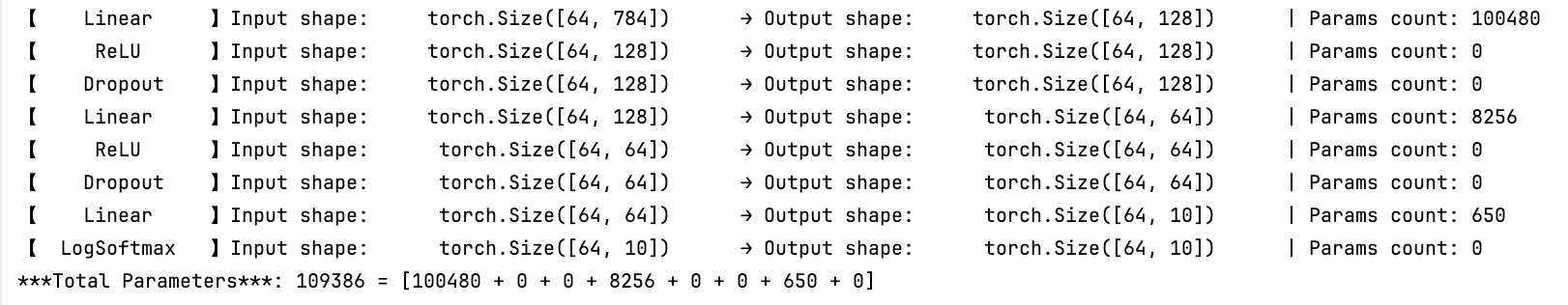
【 Linear 】Input shape: torch.Size([64, 784]) → Output shape: torch.Size([64, 128]) | Params count: 100480
【 ReLU 】Input shape: torch.Size([64, 128]) → Output shape: torch.Size([64, 128]) | Params count: 0
【 Dropout 】Input shape: torch.Size([64, 128]) → Output shape: torch.Size([64, 128]) | Params count: 0
【 Linear 】Input shape: torch.Size([64, 128]) → Output shape: torch.Size([64, 64]) | Params count: 8256
【 ReLU 】Input shape: torch.Size([64, 64]) → Output shape: torch.Size([64, 64]) | Params count: 0
【 Dropout 】Input shape: torch.Size([64, 64]) → Output shape: torch.Size([64, 64]) | Params count: 0
【 Linear 】Input shape: torch.Size([64, 64]) → Output shape: torch.Size([64, 10]) | Params count: 650
【 LogSoftmax 】Input shape: torch.Size([64, 10]) → Output shape: torch.Size([64, 10]) | Params count: 0
***Total Parameters***: 109386 = [100480 + 0 + 0 + 8256 + 0 + 0 + 650 + 0]Epoch 1, Batch 100, Loss: 1.360
Epoch 1, Batch 200, Loss: 0.689
Epoch 1, Batch 300, Loss: 0.536
Epoch 1, Batch 400, Loss: 0.495
Epoch 1, Batch 500, Loss: 0.457
Epoch 1, Batch 600, Loss: 0.434
Epoch 1, Batch 700, Loss: 0.405
Epoch 1, Batch 800, Loss: 0.397
Epoch 1, Batch 900, Loss: 0.378
Epoch 1/5 - Loss: 0.5635
Epoch 2, Batch 100, Loss: 0.352
Epoch 2, Batch 200, Loss: 0.345
Epoch 2, Batch 300, Loss: 0.354
Epoch 2, Batch 400, Loss: 0.340
Epoch 2, Batch 500, Loss: 0.309
Epoch 2, Batch 600, Loss: 0.297
Epoch 2, Batch 700, Loss: 0.325
Epoch 2, Batch 800, Loss: 0.318
Epoch 2, Batch 900, Loss: 0.307
Epoch 2/5 - Loss: 0.3257
Epoch 3, Batch 100, Loss: 0.285
Epoch 3, Batch 200, Loss: 0.290
Epoch 3, Batch 300, Loss: 0.282
Epoch 3, Batch 400, Loss: 0.289
Epoch 3, Batch 500, Loss: 0.280
Epoch 3, Batch 600, Loss: 0.271
Epoch 3, Batch 700, Loss: 0.273
Epoch 3, Batch 800, Loss: 0.272
Epoch 3, Batch 900, Loss: 0.267
Epoch 3/5 - Loss: 0.2788
Epoch 4, Batch 100, Loss: 0.257
Epoch 4, Batch 200, Loss: 0.236
Epoch 4, Batch 300, Loss: 0.269
Epoch 4, Batch 400, Loss: 0.269
Epoch 4, Batch 500, Loss: 0.264
Epoch 4, Batch 600, Loss: 0.272
Epoch 4, Batch 700, Loss: 0.255
Epoch 4, Batch 800, Loss: 0.251
Epoch 4, Batch 900, Loss: 0.254
Epoch 4/5 - Loss: 0.2578
Epoch 5, Batch 100, Loss: 0.247
Epoch 5, Batch 200, Loss: 0.219
Epoch 5, Batch 300, Loss: 0.236
Epoch 5, Batch 400, Loss: 0.226
Epoch 5, Batch 500, Loss: 0.236
Epoch 5, Batch 600, Loss: 0.250
Epoch 5, Batch 700, Loss: 0.240
Epoch 5, Batch 800, Loss: 0.240
Epoch 5, Batch 900, Loss: 0.235
Epoch 5/5 - Loss: 0.2361
Test Accuracy: 96.37%
"""
2.1.3 输出结果分析
网络结构
-
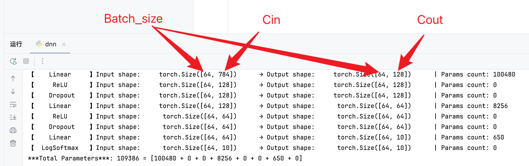
线性全连接层的参数量为: ( C i n + 1 ) × C o u t (C_{in}+1) \times C_{out} (Cin+1)×Cout,其中:
-
C i n C_{in} Cin:输入维度;
-
C o u t C_{out} Cout:输出维度;
-
其中+1是偏置量。
-
-
可以看出参数都在Linear线性层(全连接)
-
第一个线性层参数量: ( 784 + 1 ) × 128 = 100480 (784+1) \times 128 = 100480 (784+1)×128=100480;
-
第二个线性层参数量: ( 128 + 1 ) × 64 = 8256 (128+1) \times 64 = 8256 (128+1)×64=8256;
-
第三个线性层参数量: ( 64 + 1 ) × 10 = 650 (64+1) \times 10 = 650 (64+1)×10=650。
-
Epoch、Batch、Batch_size
-
Epoch:所有训练数据训练一次称为一次Epoch;
-
Batch:所有训练数据可能被分为多组进行训练,每组数据称为一个Batch;
-
Batch_size:一各Batch种元素数量称为Batch_size;例如上述网络结构中的64就是Batch_size。
-
举个例子:例如训练数据一共6400条,一次训练输入64条数据,那一次训练会有 6400 64 = 100 \frac{6400}{64} = 100 646400=100个Batch,每个Batch中有64个数据。
2.2 CNN
2.2.1 代码
# 导入必要的库
import torch
import torch.nn as nn
import torch.optim as optim
from torchvision import datasets, transforms
from torch.utils.data import DataLoader
import matplotlib.pyplot as plt# MINIST手写数字集CNN
"""
MINIST数据集:
wget https://storage.googleapis.com/cvdf-datasets/mnist/train-images-idx3-ubyte.gz
wget https://storage.googleapis.com/cvdf-datasets/mnist/train-labels-idx1-ubyte.gz
wget https://storage.googleapis.com/cvdf-datasets/mnist/t10k-images-idx3-ubyte.gz
wget https://storage.googleapis.com/cvdf-datasets/mnist/t10k-labels-idx1-ubyte.gz
"""# 设置随机种子保证可重复性
torch.manual_seed(42)# 设置计算设备(优先使用GPU)
device = torch.device("cuda" if torch.cuda.is_available() else "cpu")# -------------------- 1.数据加载与预处理 --------------------
# 定义数据预处理转换(标准化参数来自MNIST官方统计值)
transform = transforms.Compose([transforms.ToTensor(), # 将PIL图像像素[0,255]转换为[0,1]范围的Tensortransforms.Normalize((0.1307,), (0.3081,)) # 标准化到[-1,1]范围
])# 下载并加载训练集和测试集
train_dataset = datasets.MNIST(root='./data', # 数据集存储路径train=True, # 加载训练集download=True, # 自动下载数据集transform=transform # 应用定义的数据转换
)test_dataset = datasets.MNIST(root='./data',train=False, # 加载测试集download=True,transform=transform
)# 创建数据加载器(分批加载数据)
train_loader = DataLoader(train_dataset,batch_size=64, # 每批64个样本shuffle=True # 打乱训练数据顺序
)test_loader = DataLoader(test_dataset,batch_size=1000, # 测试时使用更大的批处理量shuffle=False # 测试数据无需打乱
)# -------------------- 2.定义卷积神经网络模型 --------------------
class CNN(nn.Module):def __init__(self):super(CNN, self).__init__()# 第一个卷积层:1输入通道(灰度图),10个输出通道,5x5卷积核self.conv1 = nn.Conv2d(1, 10, kernel_size=5)# 第二个卷积层:10输入通道,20个输出通道,5x5卷积核self.conv2 = nn.Conv2d(10, 20, kernel_size=5)# relu层self.relu = nn.ReLU()# 最大池化层,2x2窗口,步长2self.pool = nn.MaxPool2d(2)# 全连接层:输入维度320(计算见forward),输出10类(0-9数字)self.fc = nn.Linear(320, 10)def forward(self, x):# 输入尺寸:[batch_size, 1, 28, 28]x = self.pool(self.relu(self.conv1(x))) # -> [64,10,12,12]x = self.pool(self.relu(self.conv2(x))) # -> [64,20,4,4]x = x.view(-1, 320) # 展平处理(320=20 * 4 * 4)x = self.fc(x) # 全连接层输出return x# 实例化模型并转移到计算设备
model = CNN().to(device)# 输出网络结构
# print(model) # 通过print(model)输出模型结构,显示的是__init__中定义的层顺序,但不反映实际执行顺序
from net_structure import *
print_model_leaf_structure(model, torch.randn(64, 1, 28, 28)) # 64张图片,每张图片1个通道(灰色图像),图片尺寸28x28# -------------------- 3.定义损失函数和优化器 --------------------
criterion = nn.CrossEntropyLoss() # 交叉熵损失函数(适用于分类)
optimizer = optim.SGD(model.parameters(),lr=0.01, # 初始学习率momentum=0.5 # 动量参数加速收敛
)# -------------------- 4.训练过程 --------------------
def train(epochs):model.train() # 设置为训练模式for epoch in range(epochs):total_loss, running_loss = 0.0, 0.0for batch_idx, (data, target) in enumerate(train_loader):# 将数据转移到对应设备(CPU/GPU)data, target = data.to(device), target.to(device)# 前向传播outputs = model(data)loss = criterion(outputs, target)# 反向传播和优化optimizer.zero_grad() # 清空梯度loss.backward() # 计算梯度optimizer.step() # 更新参数# 记录损失值running_loss += loss.item()total_loss += loss.item()if batch_idx % 100 == 99: # 每100个batch打印一次print(f'Epoch {epoch + 1}, Batch {batch_idx + 1}, Loss: {running_loss / 100:.3f}')running_loss = 0# 打印每个epoch的损失print(f'Epoch {epoch + 1}/{epochs} - Loss: {total_loss / len(train_loader):.4f}')# 执行5个epoch的训练
train(epochs=5)# -------------------- 5.保存训练好的模型 --------------------
torch.save(model.state_dict(), 'mnist_cnn.pth') # 保存模型参数# -------------------- 6.模型评估 --------------------
def evaluate(new_model):new_model.eval() # 设置为评估模式correct = 0total = 0with torch.no_grad(): # 不计算梯度,节省内存for data, target in test_loader:data, target = data.to(device), target.to(device)outputs = new_model(data)_, predicted = torch.max(outputs.data, 1) # 获取预测结果(最大概率的类别)total += target.size(0)correct += (predicted == target).sum().item()accuracy = 100 * correct / totalprint(f'Test Accuracy: {accuracy:.2f}%')new_model = CNN().to(device)
# 加载保存的模型参数(演示加载过程)
new_model.load_state_dict(torch.load('mnist_cnn.pth'))
# 执行评估
evaluate(new_model)# -------------------- 7.可视化预测结果(可选) --------------------
# 获取测试集的一个batch
dataiter = iter(test_loader)
images, labels = next(dataiter)
images, labels = images.to(device), labels.to(device)# 进行预测
outputs = new_model(images)
_, preds = torch.max(outputs, 1)# 可视化前16张图片及其预测结果
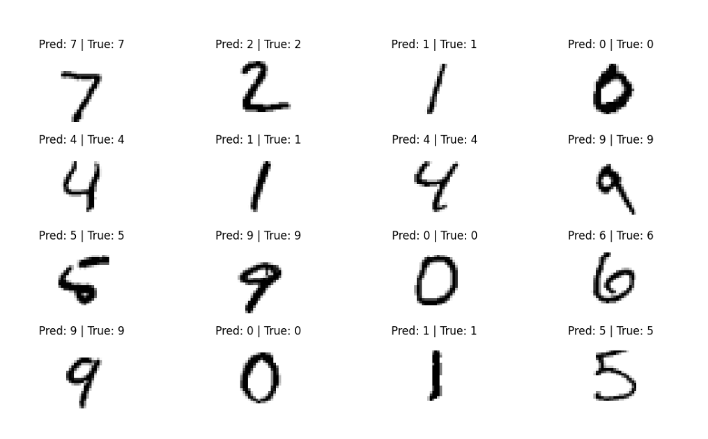
fig = plt.figure(figsize=(12, 6))
for idx in range(16):ax = fig.add_subplot(4, 4, idx + 1)img = images[idx].cpu().numpy().squeeze()ax.imshow(img, cmap='gray_r')ax.set_title(f'Pred: {preds[idx]} | True: {labels[idx]}')ax.axis('off')
plt.tight_layout()
plt.show()
2.2.2 结果
"""
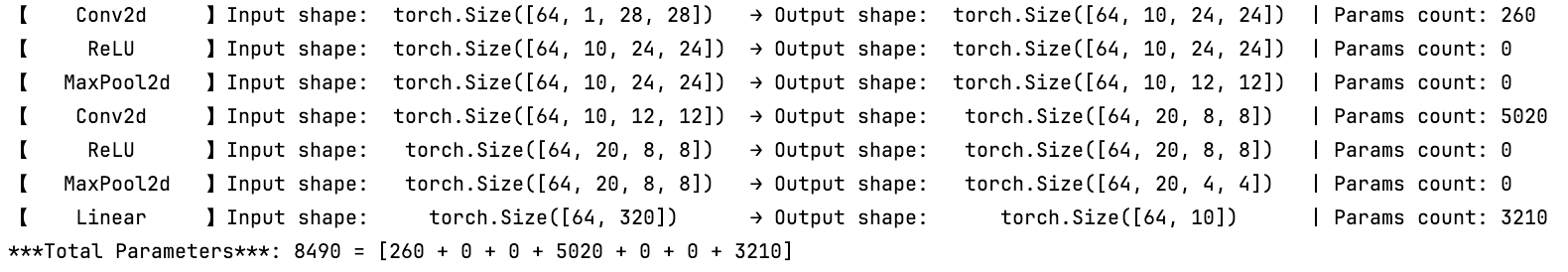
【 Conv2d 】Input shape: torch.Size([64, 1, 28, 28]) → Output shape: torch.Size([64, 10, 24, 24]) | Params count: 260
【 ReLU 】Input shape: torch.Size([64, 10, 24, 24]) → Output shape: torch.Size([64, 10, 24, 24]) | Params count: 0
【 MaxPool2d 】Input shape: torch.Size([64, 10, 24, 24]) → Output shape: torch.Size([64, 10, 12, 12]) | Params count: 0
【 Conv2d 】Input shape: torch.Size([64, 10, 12, 12]) → Output shape: torch.Size([64, 20, 8, 8]) | Params count: 5020
【 ReLU 】Input shape: torch.Size([64, 20, 8, 8]) → Output shape: torch.Size([64, 20, 8, 8]) | Params count: 0
【 MaxPool2d 】Input shape: torch.Size([64, 20, 8, 8]) → Output shape: torch.Size([64, 20, 4, 4]) | Params count: 0
【 Linear 】Input shape: torch.Size([64, 320]) → Output shape: torch.Size([64, 10]) | Params count: 3210
***Total Parameters***: 8490 = [260 + 0 + 0 + 5020 + 0 + 0 + 3210]Epoch 1, Batch 100, Loss: 1.293
Epoch 1, Batch 200, Loss: 0.383
Epoch 1, Batch 300, Loss: 0.275
Epoch 1, Batch 400, Loss: 0.223
Epoch 1, Batch 500, Loss: 0.182
Epoch 1, Batch 600, Loss: 0.161
Epoch 1, Batch 700, Loss: 0.151
Epoch 1, Batch 800, Loss: 0.142
Epoch 1, Batch 900, Loss: 0.131
Epoch 1/5 - Loss: 0.3183
Epoch 2, Batch 100, Loss: 0.114
Epoch 2, Batch 200, Loss: 0.107
Epoch 2, Batch 300, Loss: 0.114
Epoch 2, Batch 400, Loss: 0.098
Epoch 2, Batch 500, Loss: 0.100
Epoch 2, Batch 600, Loss: 0.095
Epoch 2, Batch 700, Loss: 0.090
Epoch 2, Batch 800, Loss: 0.092
Epoch 2, Batch 900, Loss: 0.086
Epoch 2/5 - Loss: 0.0998
Epoch 3, Batch 100, Loss: 0.090
Epoch 3, Batch 200, Loss: 0.072
Epoch 3, Batch 300, Loss: 0.072
Epoch 3, Batch 400, Loss: 0.079
Epoch 3, Batch 500, Loss: 0.078
Epoch 3, Batch 600, Loss: 0.072
Epoch 3, Batch 700, Loss: 0.069
Epoch 3, Batch 800, Loss: 0.083
Epoch 3, Batch 900, Loss: 0.068
Epoch 3/5 - Loss: 0.0749
Epoch 4, Batch 100, Loss: 0.063
Epoch 4, Batch 200, Loss: 0.066
Epoch 4, Batch 300, Loss: 0.063
Epoch 4, Batch 400, Loss: 0.070
Epoch 4, Batch 500, Loss: 0.061
Epoch 4, Batch 600, Loss: 0.065
Epoch 4, Batch 700, Loss: 0.058
Epoch 4, Batch 800, Loss: 0.058
Epoch 4, Batch 900, Loss: 0.055
Epoch 4/5 - Loss: 0.0625
Epoch 5, Batch 100, Loss: 0.052
Epoch 5, Batch 200, Loss: 0.057
Epoch 5, Batch 300, Loss: 0.063
Epoch 5, Batch 400, Loss: 0.052
Epoch 5, Batch 500, Loss: 0.052
Epoch 5, Batch 600, Loss: 0.066
Epoch 5, Batch 700, Loss: 0.053
Epoch 5, Batch 800, Loss: 0.051
Epoch 5, Batch 900, Loss: 0.054
Epoch 5/5 - Loss: 0.0553
Test Accuracy: 98.30%
"""
2.2.3 输出结果分析
网络结构
-
卷积层参数量: ( K h × K w × C i n + 1 ) × C o u t (K_h \times K_w \times C_{in} + 1) \times C_{out} (Kh×Kw×Cin+1)×Cout,其中
-
K h , K w K_h, K_w Kh,Kw:卷积核高宽;
-
C i n C_{in} Cin:输入通道数;
-
C o u t C_{out} Cout:输出通道数;
-
其中+1是偏置量。
-
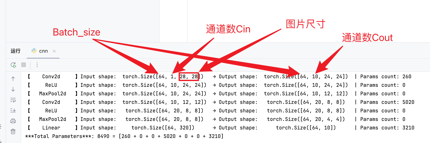
-
参数量都在卷积层和线性层:
-
第一个卷积层参数量: ( 5 × 5 × 1 + 1 ) × 10 = 260 (5 \times 5 \times 1 + 1) \times 10 = 260 (5×5×1+1)×10=260;
-
第二个卷积层参数量: ( 5 × 5 × 10 + 1 ) × 20 = 5020 (5 \times 5 \times 10 + 1) \times 20 = 5020 (5×5×10+1)×20=5020;
-
第三个卷积层参数量: ( 320 + 1 ) × 10 = 3210 (320+1) \times 10 = 3210 (320+1)×10=3210。
-
3. 绘制forward定义的模型结构
第2节中有对如下函数的使用
3.1 打印函数定义
# register_hooks 给网络注册钩子函数,用于输出网络结构,仅输出最外层结构
def register_hooks(model):def hook_fn(module, input, output):layer_name = str(module).split('(')[0]input_shape = input[0].shape if isinstance(input, tuple) else input.shapeoutput_shape = output.shapeprint(f"【{layer_name}】: Input shape: {input_shape} → Output shape: {output_shape}")hooks = []for name, layer in model.named_children():  # 遍历直接子层hook = layer.register_forward_hook(hook_fn)hooks.append(hook)return hooks# register_leaf_hooks 给网络注册钩子函数,用于输出网络结构,输出最内层结构,要求:nn中网络需要事先在__init__函数中定义
def register_leaf_hooks(model):# 定义钩子函数(捕获输入输出形状)total_params_list = []  # 初始化总参数量列表def hook_fn(module, input, output):params_count = sum(p.numel() for p in module.parameters())total_params_list.append(params_count)input_shape, output_shape = str(input[0].shape), str(output.shape)print(f"【{module.__class__.__name__:^15}】Input shape: {input_shape:^30} → Output shape: {output_shape:^30} | Params count: {params_count}")hooks = []for name, module in model.named_modules(): # forward中动态创建的层不会注册为模型的子模块,因此无法通过named_modules()遍历到,导致钩子无法绑定# 判断是否为叶子节点(无子模块)if len(list(module.children())) == 0:hook = module.register_forward_hook(hook_fn)hooks.append(hook)return hooks, total_params_list# print_model_structure 输出模型最外层结构
def print_model_structure(model, inputs):hooks = []try:hooks = register_hooks(model)if isinstance(inputs, (list, tuple)):model(*inputs)else:model(inputs)print()except Exception as e:print(e)finally:for hook in hooks:hook.remove()# print_model_structure 输出模型最内层结构
def print_model_leaf_structure(model, inputs):hooks = []try:hooks, total_params_list = register_leaf_hooks(model)if isinstance(inputs, (list, tuple)):model(*inputs)else:model(inputs)print(f"***Total Parameters***: {sum(total_params_list)} = [" + " + ".join([str(e) for e in total_params_list]) + "]\n")except Exception as e:print(e)finally:for hook in hooks:hook.remove()
3.2 打印函数的使用
注意点:
- 需要给定输入的维度,一般来说第一维是Batch_size,后面是单个数据的维度;
- 网络定义时要在__init__函数中提前定义好各层,之后直接在forward中使用__init__定义好的层,这样输出网络结构时才能够捕获到。相当于要在__init__中提前注册好各层的定义
- 例如对于上述DNN和CNN:
# 设置计算设备(优先使用GPU)
device = torch.device("cuda" if torch.cuda.is_available() else "cpu")
# 实例化模型并转移到计算设备
model = DNN().to(device)# 输出网络结构
# print(model) # 通过print(model)输出模型结构,显示的是__init__中定义的层顺序,但不反映实际执行顺序
from net_structure import *
print_model_leaf_structure(model, torch.randn(64, 1, 28, 28)) # 64张图片,每张图片1个通道(灰色图像),图片尺寸28x28